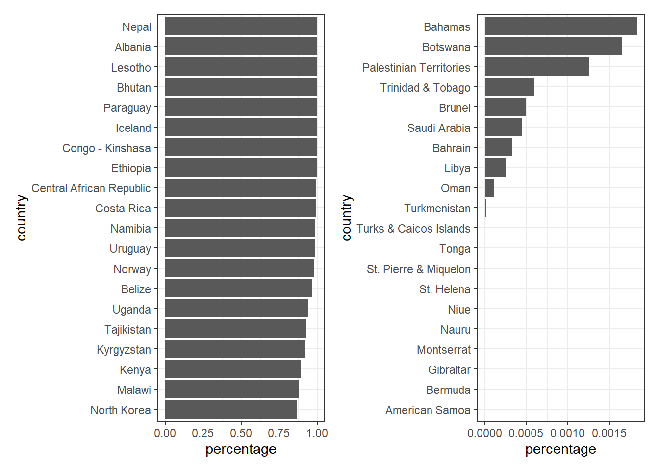
Share of renewable energy production: tops and flops

The National Bureau of Economic Research (NBER) has a a very interesting dataset on the adoption of about 200 technologies in more than 150 countries since 1800. This is theCross-country Historical Adoption of Technology (CHAT) dataset.

The following is a description of the variables

variable	class	description
variable	character	Variable name
label	character	Label for variable
iso3c	character	Country code
year	double	Year
group	character	Group (consumption/production)
category	character	Category
value	double	Value (related to label)

technology <- readr::read_csv(here::here('data/technology.csv'))

## Rows: 491636 Columns: 7
## ── Column specification ────────────────────────────────────────────────────────
## Delimiter: ","
## chr (5): variable, label, iso3c, group, category
## dbl (2): year, value
## 
## ℹ Use `spec()` to retrieve the full column specification for this data.
## ℹ Specify the column types or set `show_col_types = FALSE` to quiet this message.

#get all technologies
labels <- technology %>% 
  distinct(variable, label)

# Get country names using 'countrycode' package
technology <- technology %>% 
  filter(iso3c != "XCD") %>% 
  mutate(iso3c = recode(iso3c, "ROM" = "ROU"),
         country = countrycode(iso3c, origin = "iso3c", destination = "country.name"),
         country = case_when(
           iso3c == "ANT" ~ "Netherlands Antilles",
           iso3c == "CSK" ~ "Czechoslovakia",
           iso3c == "XKX" ~ "Kosovo",
           TRUE           ~ country))

## Warning in countrycode_convert(sourcevar = sourcevar, origin = origin, destination = dest, : Some values were not matched unambiguously: ANT, CSK, XKX

#make smaller dataframe on energy
energy <- technology %>% 
  filter(category == "Energy")

# download CO2 per capita from World Bank using {wbstats} package
# https://data.worldbank.org/indicator/EN.ATM.CO2E.PC
# co2_percap <- wb_data(country = "countries_only", 
#                       indicator = "EN.ATM.CO2E.PC", 
#                       start_date = 1970, 
#                       end_date = 2022,
#                       return_wide=FALSE) %>% 
#   filter(!is.na(value)) %>% 
#   #drop unwanted variables
#   select(-c(unit, obs_status, footnote, last_updated))

co2_percap <- read_csv(here::here("data/co2percap.csv"),skip = 4) %>% 
  janitor::clean_names()

## New names:
## Rows: 266 Columns: 67
## ── Column specification
## ──────────────────────────────────────────────────────── Delimiter: "," chr
## (4): Country Name, Country Code, Indicator Name, Indicator Code dbl (30): 1990,
## 1991, 1992, 1993, 1994, 1995, 1996, 1997, 1998, 1999, 2000, ... lgl (33): 1960,
## 1961, 1962, 1963, 1964, 1965, 1966, 1967, 1968, 1969, 1970, ...
## ℹ Use `spec()` to retrieve the full column specification for this data. ℹ
## Specify the column types or set `show_col_types = FALSE` to quiet this message.
## • `` -> `...67`

This is a very rich data set, not just for energy and CO2 data, but for many other technologies. In our case, we just need to produce a couple of graphs– at this stage, the emphasis is on data manipulation, rather than making the graphs gorgeous.

First, produce a graph with the countries with the highest and lowest % contribution of renewables in energy production. This is made up of elec_hydro, elec_solar, elec_wind, and elec_renew_other. You may want to use the patchwork package to assemble the two charts next to each other.

## `summarise()` has grouped output by 'country'. You can override using the
## `.groups` argument.